Nature of Physical World and Measurement#
Education is not the learning of facts, but the training of the mind to think" - Albert Einstein
Learning Objectives#
In this unit, the student is exposed to
• excitement generated by the discoveries in Physics
• an understanding of physical quantities of importance
• different system of units
• an understanding of errors and corrections in physics measurements
• the importance of significant figures
• usage of dimensions to check the homogeneity of physical quantities
1.1 SCIENCE-INTRODUCTION#
The word ‘science’ has its root in the Latin verb scientia, meaning “to know”. In Tamil language, it is ‘அறிவியல்’ (Ariviyal) meaning ‘knowing the truth’. The human mind is always curious to know and understand different phenomena like the bright celestial objects in nature, cyclic changes in the seasons, occurrence of rainbow, etc. The inquisitive mind looks for meaningful patterns and relations in such phenomena. Today’s modern science and technology is an offshoot of the understanding of nature. Science is the systematic organization of knowledge gained through observation, experimentation and logical reasoning. The knowledge of science dealing with non- living things is physical science
(Physics and Chemistry), and that dealing with living things is biological science (Botany, Zoology etc.).
Curiosity- driven observations of natural happenings was the origin of science. The word ‘science’ was coined only in the \(19^{\mathrm{th}}\) century. Natural philosophy was the earlier name given to science, when ancient civilization knew and practised astronomy, chemistry, human physiology and agriculture. Oral communication was the mode of conveying knowledge when writing systems were not yet developed. One of the oldest forerunners of scientific advancements, from astronomy to medicine, were the Egyptians. Scientific and mathematical excellence in India dates back to prehistoric human activity in the Indus Valley Civilization (3300 - 1300 BC(BCE).
According to part IV Article 51A (h) of Indian Constitution “It shall be the duty of every citizen of India to develop scientific temper, humanism and spirit of inquiry and reform’’. This is the aim of our Science Education.
1.1.1 The Scientific Method#
The scientific method is a step-by-step approach in studying natural phenomena and establishing laws which govern these phenomena. Any scientific method involves the following general features.
(i) Systematic observation
(ii) Controlled experimentation
(iii) Qualitative and quantitative reasoning
(iv) Mathematical modeling
(v) Prediction and verification or falsification of theories
Example
Consider a metallic rod being heated. When one end of the rod is heated, heat is felt at the other end. The following questions can be asked on this observation:
a) What happens within the rod when it is heated?
b) How does the heat reach the other end?
c) Is this effect true for all materials?
d) If heat flows through the material, is it possible to visualize heat?
The process of finding the answers to these queries is scientific investigation.
The basic phenomenon of heat is discussed in unit $8$.
1.2 PHYSICS-INTRODUCTION#
The word ‘physics’ is derived from the Greek word “Fusis”, meaning nature. The study of nature and natural phenomena is dealt within physics. Hence physics is considered as the most basic of all sciences.
Unification and Reductionism are the two approaches in studying physics. Attempting to explain diverse physical phenomena with a few concepts and laws is unification. For example, Newton’s universal law of gravitation (in unit 6) explains the motion of freely falling bodies towards the Earth, motion of planets around the Sun, motion of the Moon around the Earth, thus unifying the fundamental forces of nature.
An attempt to explain a macroscopic system in terms of its microscopic constituents is reductionism. For example, thermodynamics (unit 8) was developed to explain macroscopic properties like temperature, entropy, etc., of bulk systems. The above properties have been interpreted in terms of the molecular constituents (microscopic) of the bulk system by kinetic theory (unit 9) and statistical mechanics.
1.2.1 Branches of Physics#
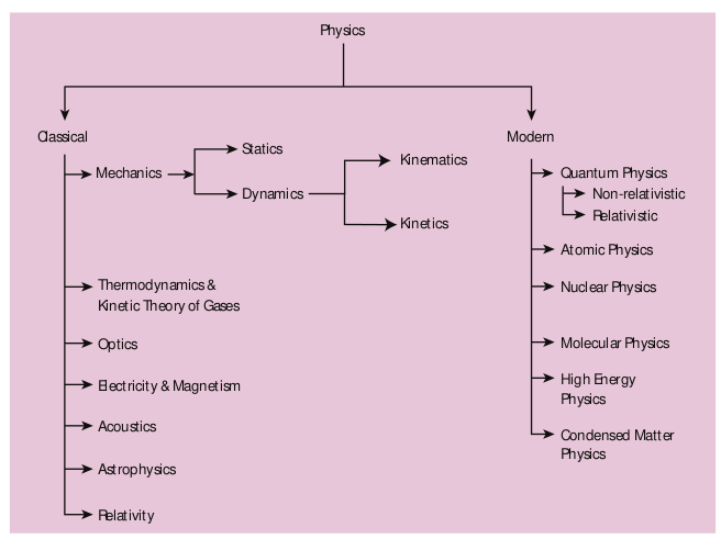
Physics as a fundamental science helps to uncover the laws of nature. The language of its expression is mathematics. In ancient times, humans lived with nature – their lifestyles were integrated with nature. They could understand the signals from the movement of the stars and other celestial bodies. They could determine the time to sow and reap by watching the sky. Thus, astronomy and mathematics were the first disciplines to be developed. The chronological development of various branches of physics is presented in Appendix A1.1. The various branches of physics are schematically shown in figure 1.1. The essential focus of different areas is given in Table 1.1.
Some of the fundamental concepts of basic areas of physics are discussed in higher secondary first year physics books volume 1 and 2. Mechanics is covered in unit 1 to 6. Unit 1 gives an idea of the development of physics along with discussion on basic elements such as measurement, units etc. Unit 2 gives the basic mathematics needed to express the impact of physical principles and their governing laws. The impact of forces acting on objects in terms of the fundamental laws of motion of Newton are very systematically covered in unit 3. Work and energy which are the basic parameters of investigation of the mechanical world are presented in unit 4. Unit 5 deals with the mechanics of rigid bodies (in contrast, objects are viewed as point objects in units 3 and 4). The basics of gravitation and its consequences are discussed in unit 6. Older branches of physics such as different properties of matter are discussed in unit 7. The impact of heat and investigations of its consequences are covered in units 8 and 9. Important features of oscillations and wave motion are covered in units 10 and 11.
| Classical Physics | Refers to traditional physics that was recognized and developed before the beginning of the 20th century. |
|---|---|
| Branch | Major focus |
| 1. Classical mechanics | The study of forces acting on bodies whether at rest or in motion |
| 2. Thermodynamics | The study of the relationship between heat and other forms of energy |
| 3. Optics | The study of light |
| 4. Electricity and magnetism | The study of electricity and magnetism and their mutual relationship |
| 5. Acoustics | The study of the production and propagation of sound waves |
| 6. Astrophysics | The branch of physics which deals with the study of the physics of astronomical bodies |
| 7. Relativity | One of the branches of theoretical physics which deals with the relationship between space, time and energy particularly with respect to objects moving in different ways |
| Modern Physics | refers to the concepts in physics that have surfaced since the beginning of the 20th century. |
|---|---|
| 1. Quantum mechanics | The study of the discrete nature of phenomena at the atomic and subatomic levels |
| 2. Atomic physics | The branch of physics which deals with the structure and properties of the atom |
| 3. Nuclear physics | The branch of physics which deals with the structure, properties and reaction of the nuclei of atoms |
| 4. Condensed matter physics | The study of the properties of condensed materials (solids, liquids and those intermediate between them and dense gas). It branches into various sub-divisions including developing fields such as nano science, photonics etc. It covers the basics of materials science, which aims at developing new material with better properties for promising applications. |
| 5. High energy physics | The study of the nature of the particles |
*Quantum mechanics is a broader approach; classical results can be reproduced in quantum mechanics also. Detailed explanation is beyond the scope of this book.
1.2.2 Scope and Excitement of Physics#
Discoveries in physics are of two types; accidental discoveries and well-analysed research outcome in the laboratory based on intuitive thinking and prediction. For example, magnetism was accidentally observed but the reason for this strange behavior of magnets was later analysed theoretically. This analysis revealed the underlying phenomena of magnetism. With this knowledge, artificial magnets were prepared in the laboratories. Theoretical predictions are the most important contribution of physics to the developments in technology and medicine. For example, the famous equation of Albert Einstein, $E = mc^2$ was a theoretical prediction in 1905 and experimentally proved in 1932 by Cockcroft and Walton. Theoretical predictions aided with recent simulation and computation procedures are widely used to identify the most suited materials for robust applications. The pharmaceutical industry uses this technique very effectively to design new drugs. Biocompatible materials for organ replacement are predicted using quantum prescriptions of physics before fabrication. Thus, experiments and theory work hand in hand complimenting one another.
Physics has a huge scope as it covers a tremendous range of magnitude of various physical quantities (length, mass, time, energy etc). It deals with systems of very large magnitude as in astronomical phenomena as well as those with very small magnitude involving electrons and protons.
- Range of time scales: astronomical scales to microscopic scales, $10^{18} , \text{s}$ to $10^{-22} , \text{s}$.
- Range of masses: from heavenly bodies to electron, $10^{55} , \text{kg}$ (mass of known observable universe) to $10^{-31} , \text{kg}$ (mass of an electron). The actual mass of an electron is $9.11 \times 10^{-31} , \text{kg}$.
The study of physics is not only educative but also exciting in many ways.
- A small number of basic concepts and laws can explain diverse physical phenomena.
- The most interesting part is the designing of useful devices based on the physical laws.
For example: i) use of robotics ii) journey to Moon and to nearby planets with controls from the ground iii) technological advances in health sciences etc.
- Carrying out new challenging experiments to unfold the secrets of nature and in verifying or falsifying the existing theories.
- Probing and understanding the science behind natural phenomena like the eclipse, and why one feels the heat when there is a fire? (or) What causes the wind, etc.
In today’s world of technological advancement, the building block of all engineering and technical education is physics which is explained with the help of mathematical tools.
1.3 PHYSICS IN RELATION TO TECHNOLOGY AND SOCIETY#
Technology is the application of the principles of physics for practical purposes. The application of knowledge for practical purposes in various fields to invent and produce useful products or to solve problems is known as technology. Thus, physics and technology can both together impact our society directly or indirectly. For example,
i. Basic laws of electricity and magnetism led to the discovery of wireless communication technology which has shrunk the world with effective communication over large distances.
ii. The launching of satellite into space has revolutionized the concept of communication.
iii. Microelectronics, lasers, computers, superconductivity and nuclear energy have comprehensively changed the thinking and living style of human beings.
Physics being a fundamental science has played a vital role in the development of all other sciences. A few examples:
1. Physics in relation to Chemistry: In physics, we study the structure of atom, radioactivity, X-ray diffraction etc. Such studies have enabled researchers in chemistry to arrange elements in the periodic table on the basis of their atomic numbers. This has further helped to know the nature of valency, chemical bonding and to understand the complex chemical structures. Inter-disciplinary branches like Physical chemistry and Quantum chemistry play important roles here.
2. Physics in relation to biology: Biological studies are impossible without a microscope designed using physics principles. The invention of the electron microscope has made it possible to see even the structure of a cell. X-ray and neutron diffraction techniques have helped us to understand the structure of nucleic acids, which help to control vital life processes. X-rays are used for diagnostic purposes. Radio-isotopes are used in radiotherapy for the cure of cancer and other diseases. In recent years, biological processes are being studied from the physics point of view.
3. Physics in relation to mathematics: Physics is a quantitative science. It is most closely related to mathematics as a tool for its development.
4. Physics in relation to astronomy: Astronomical telescopes are used to study the motion of planets and other heavenly bodies in the sky. Radio telescopes have enabled the astronomers to observe distant points of the universe. Studies of the universe are done using physical principles.
5. Physics in relation to geology: Diffraction techniques help to study the crystal structure of various rocks. Radioactivity is used to estimate the age of rocks, fossils and the age of the Earth.
6. Physics in relation to oceanography: Oceanographers seek to understand the physical and chemical processes of the oceans. They measure parameters such as temperature, salinity, current speed, gas fluxes, chemical components.
7. Physics in relation to psychology: All psychological interactions can be derived from a physical process. The movements of neurotransmitters are governed by the physical properties of diffusion and molecular motion. The functioning of our brain is related to our underlying wave-particle dualism.
Nature teaches true science with physics as an efficient tool. Science and technology should be used in a balanced manner so that they do not become weapons to destroy nature which taught us science. Global warming and other negative impacts of technology need to be checked. Safe science with moderate and appropriate use of technology is the need of this century.
The scope and opportunities for higher education in physics and various fellowships offered is given in the beginning of the book.
1.4 MEASUREMENT#
“When you can measure what you are speaking about and can express it in numbers, you know something about it; but when you cannot express it in numbers, your knowledge is of a meager and unsatisfactory kind” — Lord Kelvin
The comparison of any physical quantity with its standard unit is known as measurement.
Measurement is the basis of all scientific studies and experimentation. It plays an important role in our daily life. Physics is a quantitative science and physicists always deal with numbers which are the measurement of physical quantities.
1.4.1 Definition of Physical Quantity#
Quantities that can be measured, and in terms of which, laws of physics are described are called physical quantities. Examples are length, mass, time, force, energy, etc.
1.4.2 Types of Physical Quantities#
Physical quantities are classified into two types. They are fundamental and derived quantities.
Fundamental or base quantities are quantities which cannot be expressed in terms of any other physical quantities. These are length, mass, time, electric current, temperature, luminous intensity and amount of substance.
Quantities that can be expressed in terms of fundamental quantities are called derived quantities. For example, area, volume, velocity, acceleration, force, etc.
1.4.3 Definition of Unit and its Types#
The process of measurement is basically a process of comparison. To measure a quantity, we always compare it with some reference standard. For example, when we state that a rope is 10 meter long, it is to say that it is 10 times as long as an object whose length is defined as 1 metre. Such a standard is known as the unit of the quantity. Here 1 metre is the unit of the quantity ’length’.
An arbitrarily chosen standard of measurement of a quantity, which is accepted internationally is called unit of the quantity.
The units in which the fundamental quantities are measured are called fundamental or base units and the units of measurement of all other physical quantities, which can be obtained by a suitable multiplication or division of powers of fundamental units, are called derived units.
1.4.4 Different types of Measurement Systems#
A complete set of units which is used to measure all kinds of fundamental and derived quantities is called a system of units. Here are the common system of units used in mechanics:
(a) the f.p.s. system is the British Engineering system of units, which uses foot, pound and second as the three basic units for measuring length, mass and time respectively.
(b) The c.g.s system is the Gaussian system, which uses centimeter, gram and second as the three basic units for measuring length, mass and time respectively.
(c) The m.k.s system is based on metre, kilogram and second as the three basic units for measuring length, mass and time respectively.
Did you know? The cgs, mks and SI are metric or decimal system of units. The fps system is not a metric system.
1.4.5 SI Unit System#
The system of units used by scientists and engineers around the world is commonly called the metric system but, since 1960, it has been known officially as the International System, or SI (the abbreviation for its French name, Système International). The SI with a standard scheme of symbols, units and abbreviations, were developed and recommended by the General Conference on Weights and Measures in 1971 for international usage in scientific, technical, industrial and commercial work. The advantages of the SI system are,
i) This system makes use of only one unit for one physical quantity, which means a rational system of units.
ii) In this system, all the derived units can be easily obtained from basic and supplementary units, which means it is a coherent system of units.
iii) It is a metric system which means that multiples and submultiples can be expressed as powers of 10.
In SI, there are seven fundamental units as given in Table 1.2
Table 1.2 SI Base Quantities and Units
| Base Quantity | Units | Unit Symbol | Definition |
|---|---|---|---|
| Length | metre | m | One metre is the length of the path travelled by light in vacuum in $1/299{,}792{,}458$ of a second (1983) |
| Mass | kilogram | kg | One kilogram is the mass of the prototype cylinder of platinum iridium alloy (whose height is equal to its diameter), preserved at the International Bureau of Weights and Measures at Serves, near Paris, France. (1901) |
| Time | second | s | One second is the duration of $9{,}192{,}631{,}770$ periods of radiation corresponding to the transition between the two hyperfine levels of the ground state of Cesium-133 atom. (1967) |
| Electric current | ampere | A | One ampere is the constant current, which when maintained in each of the two straight parallel conductors of infinite length and negligible cross section, held one metre apart in vacuum shall produce a force per unit length of $2 \times 10^{-7} , \text{N/m}$ between them. (1948) |
| Temperature | kelvin | K | One kelvin is the fraction $\frac{1}{273.16}$ of the thermodynamic temperature of the triple point* of the water. (1967) |
| Amount of substance | mole | mol | One mole is the amount of substance which contains as many elementary entities as there are atoms in $0.012 , \text{kg}$ of pure carbon-12. (1971) |
| Luminous intensity | candela | cd | One candela is the luminous intensity in a given direction, of a source that emits monochromatic radiation of frequency $5.4 \times 10^{14} , \text{Hz}$ and that has a radiant intensity of $\frac{1}{683}$ watt/steradian in that direction. (1979) |
*Triple point of water is the temperature at which saturated vapour, pure water and melting ice are all in equilibrium. The triple point temperature of water is $273.16 , \text{K}$.
Table 1.3 Derived Quantities and their Units
| Physical quantity | Expression | Unit |
|---|---|---|
| Plane angle | $\text{arc} / \text{radius}$ | rad |
| Solid angle | $\text{surface area} / \text{radius}^2$ | sr |
| Area | $\text{length} \times \text{breadth}$ | $\text{m}^2$ |
| Volume | $\text{area} \times \text{height}$ | $\text{m}^3$ |
| Velocity | $\text{displacement} / \text{time}$ | $\text{m} , \text{s}^{-1}$ |
| Acceleration | $\text{velocity} / \text{time}$ | $\text{m} , \text{s}^{-2}$ |
| Angular velocity | $\text{angular displacement} / \text{time}$ | $\text{rad} , \text{s}^{-1}$ |
| Angular acceleration | $\text{angular velocity} / \text{time}$ | $\text{rad} , \text{s}^{-2}$ |
| Density | $\text{mass} / \text{volume}$ | $\text{kg} , \text{m}^{-3}$ |
| Linear momentum | $\text{mass} \times \text{velocity}$ | $\text{kg} , \text{m} , \text{s}^{-1}$ |
| Moment of inertia | $\text{mass} \times (\text{distance})^2$ | $\text{kg} , \text{m}^2$ |
| Force | $\text{mass} \times \text{acceleration}$ | $\text{kg} , \text{m} , \text{s}^{-2}$ or $\text{N}$ |
| Pressure | $\text{force} / \text{area}$ | $\text{N} , \text{m}^{-2}$ or $\text{Pa}$ |
| Energy (work) | $\text{force} \times \text{distance}$ | $\text{N} , \text{m}$ or $\text{J}$ |
| Power | $\text{Work} / \text{time}$ | $\text{J} , \text{s}^{-1}$ or $\text{watt} , (\text{W})$ |
| Impulse | $\text{force} \times \text{time}$ | $\text{N} , \text{s}$ |
| Surface tension | $\text{force} / \text{length}$ | $\text{N} , \text{m}^{-1}$ |
| Moment of force (torque) | $\text{force} \times \text{distance}$ | $\text{N} , \text{m}$ |
| Electric charge | $\text{current} \times \text{time}$ | $\text{A} , \text{s}$ or $\text{C}$ |
| Current density | $\text{current} / \text{area}$ | $\text{A} , \text{m}^{-2}$ |
| Magnetic induction | $\text{force} / (\text{current} \times \text{length})$ | $\text{N} , \text{A}^{-1} , \text{m}^{-1}$ or $\text{tesla}$ |
| Force constant | $\text{force} / \text{displacement}$ | $\text{N} , \text{m}^{-1}$ |
| Planck’s constant | $\text{energy of photon} / \text{frequency}$ | $\text{J} , \text{s}$ |
| Specific heat (S) | $\text{heat energy} / (\text{mass} \times \text{temperature})$ | $\text{J} , \text{kg}^{-1} , \text{K}^{-1}$ |
| Boltzmann constant (k) | $\text{energy} / \text{temperature}$ | $\text{J} , \text{K}^{-1}$ |
Note:
$$ \pi \, \text{radian} = 180^\circ $$$$ 1 \, \text{radian} = \frac{180}{\pi} \approx \frac{180 \times 7}{22} \approx 57^\circ 27'' $$Also, $1^\circ$ (degree of arc) = $60’$ (minute of arc) and $1’$ (minute of arc) = $60’’$ (seconds of arc)
Relations between radian, degree and minutes:
$$ \begin{array}{l} 1^\circ = \frac{\pi}{180} \, \text{rad} = 1.744 \times 10^{-2} \, \text{rad} \\ \\ 1' = \frac{1}{60} \times 1.744 \times 10^{-2} \, \text{rad} = 2.906 \times 10^{-4} \, \text{rad} \approx 2.91 \times 10^{-4} \, \text{rad} \\ \\ 1'' = \frac{1}{3600} \times 1.744 \times 10^{-2} \, \text{rad} \approx 4.84 \times 10^{-6} \, \text{rad} \end{array} $$1.5 MEASUREMENT OF BASIC QUANTITIES#
1.5.1 Measurement of Length#
The Radian (rad): One radian is the angle subtended at the centre of a circle by an arc equal in length to the radius of the circle.
The Steradian (sr): One steradian is the solid angle subtended at the centre of a sphere, by that surface of the sphere, which is equal in area, to the square of radius of the sphere.
The concept of length in physics is related to the concept of distance in everyday life. Length is defined as the distance between any two points in space. The SI unit of length is metre. The objects of our interest vary widely in sizes. For example, large objects like the galaxy, stars, Sun, Earth, Moon etc., and their distances constitute a macrocosm. It refers to a large world, in which both objects and distances are large. On the contrary, objects like molecules, atoms, proton, neutron, electron, bacteria etc., and their distances constitute microcosm, which means a small world in which both objects and distances are small-sized.
Distances ranging from $10^{-5}$ m to $10^{2}$ m can be measured by direct methods. For example, a metre scale can be used to measure the distance from $10^{-3}$ m to $1$ m, vernier calipers up to $10^{-4}$ m, a screw gauge up to $10^{-5}$ m and so on. The atomic and astronomical distances cannot be measured by any of the above mentioned direct methods. Hence, to measure the very small and the very large distances, indirect methods have to be devised and used. In Table 1.4, a list of powers of $10$ (both positive and negative powers) is given. Prefixes for each power are also mentioned. These prefixes are used along with units of length, and of mass.
Did you know? The supplementary quantities of plane and solid angle were converted into Derived quantities in 1995 (GCWM)
Table 1.4 Prefixes for Powers of Ten
| Multiple | Prefix | Symbol | Sub multiple | Prefix | Symbol |
|---|---|---|---|---|---|
| $10^{1}$ | deca | da | $10^{-1}$ | deci | d |
| $10^{2}$ | hecto | h | $10^{-2}$ | centi | c |
| $10^{3}$ | kilo | k | $10^{-3}$ | milli | m |
| $10^{6}$ | mega | M | $10^{-6}$ | micro | $\mu$ |
| $10^{9}$ | giga | G | $10^{-9}$ | nano | n |
| $10^{12}$ | tera | T | $10^{-12}$ | pico | p |
| $10^{15}$ | peta | P | $10^{-15}$ | femto | f |
| $10^{18}$ | exa | E | $10^{-18}$ | atto | a |
| $10^{21}$ | zetta | Z | $10^{-21}$ | zepto | z |
| $10^{24}$ | yotta | Y | $10^{-24}$ | yocto | y |
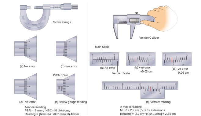
i) Measurement of small distances: screw gauge and vernier caliper
Screw gauge: The screw gauge is an instrument used for measuring accurately the dimensions of objects up to a maximum of about $50$ mm. The principle of the instrument is the magnification of linear motion using the circular motion of a screw. The least count of the screw gauge is $0.01$ mm.
Vernier caliper: A vernier caliper is a versatile instrument for measuring the dimensions of an object namely diameter of a hole, or a depth of a hole. The least count of the vernier caliper is $0.01$ cm.
ii) Measurement of large distances
For measuring larger distances such as the height of a tree, distance of the Moon or a planet from the Earth, some special methods are adopted. Triangulation method, parallax method and radar method are used to determine very large distances.
Triangulation method for the height of an accessible object
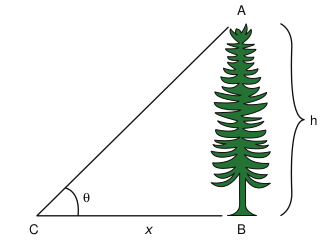
Let $AB = h$ be the height of the tree or tower to be measured. Let $C$ be the point of observation at distance $x$ from $B$. Place a range finder at $C$ and measure the angle of elevation, $\angle ACB = \theta$ as shown in Figure 1.3. From right angled triangle $ABC$,
$$ \tan \theta = \frac{AB}{BC} = \frac{h}{x} $$(or)
$$ \text{height } h = x \tan \theta $$Knowing the distance $x$, the height $h$ can be determined.
Range and order of lengths of various objects are listed in Table 1.5
EXAMPLE 1.1
From a point on the ground, the top of a tree is seen to have an angle of elevation $60^\circ$. The distance between the tree and a point is $50$ m. Calculate the height of the tree?
Solution
Angle $\theta = 60^\circ$
The distance between the tree and a point $x = 50$ m
Height of the tree $h = ?$
For triangulation method $\tan \theta = \frac{h}{x}$
$$ h = x \tan \theta = 50 \times \tan 60^\circ = 50 \times 1.732 $$$$ h = 86.6 \text{ m} $$The height of the tree is $86.6$ m.
Parallax method
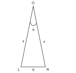
Very large distances, such as the distance of a planet or a star from the Earth can be measured by the parallax method. Parallax is the name given to the apparent change in the position of an object with respect to the background, when the object is seen from two different positions. The distance between the two positions (i.e., points of observation) is called the basis ($b$). Consider any object at the location $O$ (Figure 1.4).
Let $L$ and $R$ represent the positions of the left and right eyes of the observer respectively.
The object ($O$) is viewed with the left eye ($L$) keeping the right eye closed and the same object ($O$) is viewed with the right eye ($R$) keeping the left eye closed.
In Figure 1.4, $LO$ and $RO$ are the lines drawn from the positions of the left and right eyes to the object. These two lines make an angle $\theta$ at $O$. This angle $\theta$ is called the angle of parallax.
$OL$ and $OR$ are considered as the radii ($x$) of a circle. For astronomical calculation, the distance $LR = b$ (basis) can be treated as an arc of this circle, then
$$ OL = OR = x $$as $LR = b$
$$ \theta = \frac{b}{x} $$Knowing $b$ and $\theta$, $x$ can be calculated which is approximately the distance of the object from the observer.
If the object is the Moon or any nearby star, then the angle $\theta$ will be too small due to the large astronomical distance and the place of observation. In this case, the two points of observation should be sufficiently spaced on the surface of the Earth.
Determination of distance of Moon from Earth
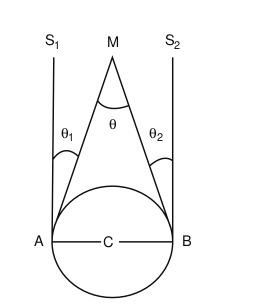
In Figure 1.5, $C$ is the centre of the Earth. $A$ and $B$ are two diametrically opposite places on the surface of the Earth. From $A$ and $B$, the parallaxes $\theta_1$ and $\theta_2$ respectively of Moon $M$ with respect to some distant star are determined with the help of an astronomical telescope. Thus, the total parallax of the Moon subtended on Earth $\angle AMB = \theta_1 + \theta_2 = \theta$.
If $\theta$ is measured in radians, then
$$ \theta = \frac{AB}{AM} \quad ; \quad AM \approx MC \text{ (AM is approximately equal to MC)} $$$$ \theta = \frac{AB}{MC} \quad \text{or} \quad MC = \frac{AB}{\theta} ; $$Knowing the values of $AB$ and $\theta$, we can calculate the distance $MC$ of Moon from the Earth.
EXAMPLE 1.2
The Moon subtends an angle of $1^\circ 55’$ at the base line equal to the diameter of the Earth. What is the distance of the Moon from the Earth? (Radius of the Earth is $6.4 \times 10^{6}$ m)
Solution
Angle $\theta = 1^\circ 55’ = 115’ = (115 \times 60)’’ \times (4.85 \times 10^{-6})$ rad
$$ \theta = 3.34 \times 10^{-2} \text{ rad} $$(since $1’’ = 4.85 \times 10^{-6}$ rad)
Radius of the Earth $= 6.4 \times 10^{6}$ m
From Figure 1.5, $AB$ is the diameter of the Earth ($b$) $= 2 \times 6.4 \times 10^{6}$ m
Distance of the Moon from the Earth $x = ?$
$$ x = \frac{b}{\theta} = \frac{2 \times 6.4 \times 10^{6}}{3.34 \times 10^{-2}} $$$$ x = 3.83 \times 10^{8} \text{ m} $$RADAR method
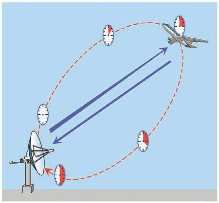
The word RADAR stands for radio detection and ranging. A radar can be used to measure accurately the distance of a nearby planet such as Mars. In this method, radio waves are sent from transmitters which, after reflection from the planet, are detected by the receiver. By measuring the time interval ($t$) between the instants the radio waves are sent and received, the distance of the planet can be determined as
Speed $= \frac{\text{distance travelled}}{\text{time taken}}$ (Speed is explained in unit 2)
$$ \text{Distance } (d) = \frac{\text{Speed of radio waves} \times \text{time taken}}{2} d = \frac{v \times t}{2} $$where $v$ is the speed of the radio wave. As the time taken ($t$) is for the distance covered during the forward and backward path of the radio waves, it is divided by $2$ to get the actual distance of the object. This method can also be used to determine the height at which an aeroplane flies from the ground.
EXAMPLE 1.3
A RADAR signal is beamed towards a planet and its echo is received $7$ minutes later. If the distance between the planet and the Earth is $6.3 \times 10^{10}$ m, calculate the speed of the signal.
Solution
The distance of the planet from the Earth $d = 6.3 \times 10^{10}$ m
Time $t = 7$ minutes $= 7 \times 60$ s
The speed of signal $v = ?$
The speed of signal
$$ v = \frac{2d}{t} = \frac{2 \times 6.3 \times 10^{10}}{7 \times 60} = 3 \times 10^{8} \text{ m/s} $$Table 1.5 Range and Order of Lengths
| Size of objects and distances | Length (m) |
|---|---|
| Distance to the boundary of observable universe | $10^{26}$ |
| Distance to the Andromeda galaxy | $10^{22}$ |
| Size of our galaxy | $10^{21}$ |
| Distance from Earth to the nearest star (other than the Sun) | $10^{16}$ |
| Average radius of Pluto’s orbit | $10^{12}$ |
| Distance of the Sun from the Earth | $10^{11}$ |
| Distance of Moon from the Earth | $10^{8}$ |
| Radius of the Earth | $10^{7}$ |
| Height of the Mount Everest above sea level | $10^{4}$ |
| Length of a football field | $10^{2}$ |
| Thickness of a paper | $10^{-4}$ |
| Diameter of a red blood cell | $10^{-5}$ |
| Wavelength of light | $10^{-7}$ |
| Length of typical virus | $10^{-8}$ |
| Diameter of the hydrogen atom | $10^{-10}$ |
| Size of atomic nucleus | $10^{-14}$ |
| Diameter of a proton | $10^{-15}$ |
Some Common Practical Units
(i) Fermi $= 1 \text{ fm} = 10^{-15}$ m
(ii) $1$ angstrom $= 1 \text{ Å} = 10^{-10}$ m
(iii) $1$ nanometer $= 1 \text{ nm} = 10^{-9}$ m
(iv) $1$ micron $= 1 \ \mu\text{m} = 10^{-6}$ m
(v) $1$ Light year (Distance travelled by light in vacuum in one year)
$1 \text{ Light Year} = 9.467 \times 10^{15}$ m
(vi) $1$ astronomical unit (the mean distance of the Earth from the Sun)
$1 \text{ AU} = 1.496 \times 10^{11}$ m
(vii) $1$ parsec (Parallactic second) (Distance at which an arc of length $1$ AU subtends an angle of $1$ second of arc)
$1 \text{ parsec} = 3.08 \times 10^{16}$ m $= 3.26$ light year
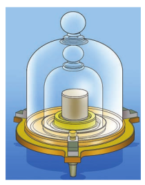
Figure 1.7 The international 1 kg standard of mass, aplatinum-iridium (9:1) cylinder 3.9 cm in height anddiameter.
Did ypu know? Why is the cylinder used in defining kilogram made up of platinum-iridium alloy?
This is because the platinum-iridium alloy is least affected by environment and time.
Chandrasekhar Limit (CSL) is the largest practical unit of mass.
$1 \text{ CSL} = 1.4$ times the mass of the Sun
The smallest practical unit of time is Shake.
$1 \text{ Shake} = 10^{-8}$ s
1.5.2 Measurement of Mass#
Mass is a property of matter. It does not depend on temperature, pressure and location of the body in space. Mass of a body is defined as the quantity of matter contained in a body. The SI unit of mass is kilogram (kg). The masses of objects which we shall study in this course vary over a wide range. These may vary from a tiny mass of electron ($9.11 \times 10^{-31}$ kg) to the huge mass of the known universe ($=10^{55}$ kg). The order of masses of various objects is shown in Table 1.6.
Ordinarily, the mass of an object is determined in kilograms using a common balance like the one used in a grocery shop. For measuring larger masses like that of planets, stars etc., we make use of gravitational methods. For measurement of small masses of atomic/subatomic particles etc., we make use of a mass spectrograph. Some of the weighing balances commonly used are common balance, spring balance, electronic balance, etc.
Table 1.6 Range of masses
| Object | Order of mass (kg) |
|---|---|
| Electron | $10^{-30}$ |
| Proton or Neutron | $10^{-27}$ |
| Uranium atom | $10^{-25}$ |
| Red blood corpuscle | $10^{-14}$ |
| A cell | $10^{-10}$ |
| Dust particle | $10^{-9}$ |
| Raindrop | $10^{-6}$ |
| Mosquito | $10^{-5}$ |
| Grape | $10^{-3}$ |
| Frog | $10^{-1}$ |
| Human | $10^{2}$ |
| Car | $10^{3}$ |
| Ship | $10^{5}$ |
| Moon | $10^{23}$ |
| Earth | $10^{25}$ |
| Sun | $10^{30}$ |
| Milky way | $10^{41}$ |
| Observable Universe | $10^{55}$ |
1.5.3 Measurement of Time Intervals#
“Time flows uniformly forward” — Sir Isaac Newton
“Time is what a clock reads” — Albert Einstein
A clock is used to measure the time interval. An atomic standard of time, is based on the periodic vibration produced in a Cesium atom. Some of the clocks developed later are electric oscillators, electronic oscillators, solar clock, quartz crystal clock, atomic clock, decay of elementary particles, radioactive dating etc. The order of time intervals are tabulated in Table 1.7.
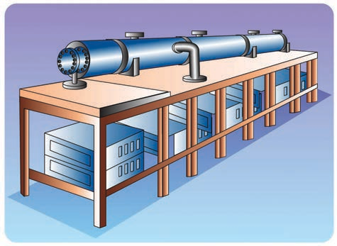
Figure 1.8 The atomic clock, which keeps time on the basis of radiation from cesium atoms is accurate to about three millionths of a second per year.
Table 1.7 Order of Time Intervals
| Event | Order of time interval (s) |
|---|---|
| Lifespan of the most unstable particle | $10^{-24}$ |
| Time taken by light to cross a distance of nuclear size | $10^{-22}$ |
| Period of X-rays | $10^{-19}$ |
| Time period of electron in hydrogen atom | $10^{-15}$ |
| Period of visible light waves | $10^{-15}$ |
| Time taken by visible light to cross through a window pane | $10^{-8}$ |
| Lifetime of an excited state of an atom | $10^{-8}$ |
| Period of radio waves | $10^{-6}$ |
| Time period of audible sound waves | $10^{-3}$ |
| Wink of an eye | $10^{-1}$ |
| Time interval between two successive heart beats | $10^{0}$ |
| Travel time of light from Moon to Earth | $10^{0}$ |
| Travel time of light from Sun to Earth | $10^{2}$ |
| Halflife time of a free neutron | $10^{3}$ |
| Time period of a satellite | $10^{4}$ |
| Time period of rotation of Earth around its axis (one day) | $10^{5}$ |
| Time period of revolution of Earth around the Sun (one year) | $10^{7}$ |
| Average life of a human being | $10^{9}$ |
| Age of Egyptian pyramids | $10^{11}$ |
| Age of Universe | $10^{17}$ |
1.6 THEORY OF ERRORS#
The foundation of all experimental science and technology is measurement. The result obtained from any measurement will contain some uncertainty. Such an uncertainty is termed error. Any calculation made using the measured values will also have an error. It is not possible to make exact measurements in an experiment.
In measurements, two different terms, accuracy and precision, are used and need to be distinguished at this stage. Accuracy refers to how far we are from the true value, and precision refers to how well we measure.
In India, the National Physical Laboratory (New Delhi) has the responsibility of maintenance and improvement of physical standards of length, mass, time, etc.
1.6.1 Accuracy and Precision#
Let us say, you know your true height is exactly $5'9’’$. You first measure your height with a yardstick and get the value $5'0’’$. Your measurement is hence not accurate. Now you measure your height with a laser yardstick and get $5'9’’$ as the value. Now your measurement is accurate. The true value is also called theoretical value. The level of accuracy required for each application varies greatly. Highly accurate data can be very difficult to produce and compile. For example, if you consistently measure your height as $5'0’’$ with a yard stick, your measurements are precise. The level of precision required for different applications varies to a great extent. Engineering projects such as road and utility construction require very precise information measured to the millimeter or one-tenth of an inch.
If a measurement is precise, that does not necessarily mean that it is accurate. However, if the measurement is consistently accurate, it is also precise.
For example, if the temperature outside a building is $40^\circ$C as measured by a weather thermometer and if the real outside temperature is $40^\circ$C, the thermometer is accurate. If the thermometer consistently registers this exact temperature in a row, the thermometer is precise.
Consider another example. Let the temperature of a refrigerator repeatedly measured by a thermometer be given as $10.4^\circ$C, $10.2^\circ$C, $10.3^\circ$C, $10.1^\circ$C, $10.2^\circ$C, $10.1^\circ$C, $10.1^\circ$C, $10.1^\circ$C. However, if the real temperature inside the refrigerator is $9^\circ$C, we say that the thermometer is not accurate (it is almost one degree off the true value), but since all the measured values are close to $10^\circ$C, hence it is precise.
A visual example: Target shooting is an example which explains the difference between accuracy and precision. In Figure 1.9 (a), the shots are focused so as to reach the bull’s eye (midpoint), but the arrows have reached only around this point. Hence the shots are not accurate and also not precise.
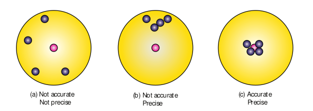
In Figure 1.9 (b), all the shots are close to each other but not at the central point. Hence the shots are said to be precise but not accurate. In Figure 1.9 (c), the shots are closer and also at the central point. Hence the shots are both precise and accurate.
A numerical example: The true value of a certain length is nearly $5.678$ cm. In one experiment, using a measuring instrument of resolution $0.1$ cm, the measured value is found to be $5.5$ cm. In another experiment using a measuring instrument of greater resolution, say $0.01$ cm, the length is found to be $5.38$ cm. We find that the first measurement is more accurate as it is closer to the true value, but it has lesser precision. On the contrary, the second measurement is less accurate, but it is more precise.
1.6.2 Errors in Measurement#
The uncertainty in a measurement is called an error. Random error, systematic error and gross error are the three possible errors.
i) Systematic errors
Systematic errors are reproducible inaccuracies that are consistently in the same direction. These occur often due to a problem that persists throughout the experiment. Systematic errors can be classified as follows:
- Instrumental errors: When an instrument is not calibrated properly at the time of manufacture, instrumental errors may arise. If a measurement is made with a meter scale whose end is worn out, the result obtained will have errors. These errors can be corrected by choosing the instrument carefully.
- Imperfections in experimental technique or procedure: These errors arise due to the limitations in the experimental arrangement. As an example, while performing experiments with a calorimeter, if there is no proper insulation, there will be radiation losses. This results in errors and to overcome these, necessary correction has to be applied.
- Personal errors: These errors are due to individuals performing the experiment, may be due to incorrect initial setting up of the experiment or carelessness of the individual making the observation due to improper precautions.
- Errors due to external causes: The change in the external conditions during an experiment can cause error in measurement. For example, changes in temperature, humidity, or pressure during measurements may affect the result of the measurement.
- Least count error: Least count is the smallest value that can be measured by the measuring instrument, and the error due to this measurement is least count error. The instrument’s resolution hence is the cause of this error. Least count error can be reduced by using a high precision instrument for the measurement.
ii) Random errors
Random errors may arise due to random and unpredictable variations in experimental conditions like pressure, temperature, voltage supply etc. Errors may also be due to personal errors by the observer who performs the experiment. Random errors are sometimes called “chance error”. When different readings are obtained by a person every time he repeats the experiment, personal error occurs. For example, consider the case of the thickness of a wire measured using a screw gauge. The readings taken may be different for different trials. In this case, a large number of measurements are made and then the arithmetic mean is taken.
If $n$ number of trial readings are taken in an experiment, and the readings are $a_1, a_2, a_3, \ldots, a_n$. The arithmetic mean is:
$$ a_m = \frac{a_1 + a_2 + a_3 + \ldots + a_n}{n} \tag{1.1} $$or
$$ a_m = \frac{1}{n} \sum_{i=1}^{n} a_i \tag{1.2} $$Usually this arithmetic mean is taken as the best possible true value of the quantity.
Certain procedures to be followed to minimize experimental errors, along with examples are shown in Table 1.8.
iii) Gross Error
The error caused due to the shear carelessness of an observer is called gross error. For example:
(i) Reading an instrument without setting it properly.
(ii) Taking observations in a wrong manner without bothering about the sources of errors and the precautions.
(iii) Recording wrong observations.
(iv) Using wrong values of the observations in calculations.
These errors can be minimized only when an observer is careful and mentally alert.
Table 1.8 Minimizing Experimental Error
| Type of error | Example | How to minimize it |
|---|---|---|
| Random error | Suppose you measure the mass of a ring three times using the same balance and get slightly different values: $15.46$ g, $15.42$ g, $15.44$ g | Take more data. Random errors can be evaluated through statistical analysis and can be reduced by averaging over a large number of observations. |
| Systematic error | Suppose the cloth tape measure that you use to measure the length of an object has been stretched out from years of use. (As a result all of the length measurements are not correct). | Systematic errors are difficult to detect and cannot be analysed statistically, because all of the data is in the same direction (either too high or too low). |
1.6.3 Error Analysis#
i) Absolute Error
The magnitude of difference between the true value and the measured value of a quantity is called absolute error. If $a_1, a_2, a_3, \ldots, a_n$ are the measured values of any quantity $a$ in an experiment performed $n$ times, then the arithmetic mean of these values is called the true value ($a_m$) of the quantity.
$$ a_m = \frac{a_1 + a_2 + a_3 + \ldots + a_n}{n} = \frac{1}{n} \sum_{i=1}^{n} a_i $$The absolute error in measured values is given by:
$$ \begin{array}{l} |\Delta a_1| = |a_m - a_1| \\ |\Delta a_2| = |a_m - a_2| \\ \vdots \\ |\Delta a_n| = |a_m - a_n| \end{array} $$ii) Mean Absolute Error
The arithmetic mean of absolute errors in all the measurements is called the mean absolute error.
$$ \Delta a_m = \frac{|\Delta a_1| + |\Delta a_2| + |\Delta a_3| + \ldots + |\Delta a_n|}{n} = \frac{1}{n} \sum_{i=1}^{n} |\Delta a_i| $$If $a_m$ is the true value and $\Delta a_m$ is the mean absolute error then the magnitude of the quantity may lie between $a_m + \Delta a_m$ and $a_m - \Delta a_m$.
iii) Relative Error
The ratio of the mean absolute error to the mean value is called relative error. This is also called as fractional error. Thus
$$ \text{Relative error} = \frac{\text{Mean absolute error}}{\text{Mean value}} = \frac{\Delta a_m}{a_m} $$Relative error expresses how large the absolute error is compared to the total size of the object measured. For example, a driver’s speedometer shows that his car is travelling at $60$ km h$^{-1}$ when it is actually moving at $62$ km h$^{-1}$. Then absolute error of speedometer is $62 - 60 = 2$ km h$^{-1}$. Relative error of the measurement is $2$ km h$^{-1} / 62$ km h$^{-1} = 0.032$.
iv) Percentage Error
The relative error expressed as a percentage is called percentage error.
$$ \text{Percentage error} = \frac{\Delta a_m}{a_m} \times 100\% $$A percentage error very close to zero means one is close to the targeted value, which is good and acceptable. It is always necessary to understand whether error is due to impression of equipment used or a mistake in the experimentation.
EXAMPLE 1.4
In a series of successive measurements in an experiment, the readings of the period of oscillation of a simple pendulum were found to be $2.63$ s, $2.56$ s, $2.42$ s, $2.71$ s and $2.80$ s. Calculate (i) the mean value of the period of oscillation (ii) the absolute error in each measurement (iii) the mean absolute error (iv) the relative error (v) the percentage error. Express the result in proper form.
Solution
$t_1 = 2.63$ s, $t_2 = 2.56$ s, $t_3 = 2.42$ s, $t_4 = 2.71$ s, $t_5 = 2.80$ s
(i)
$$ T_m = \frac{t_1 + t_2 + t_3 + t_4 + t_5}{5} = \frac{2.63 + 2.56 + 2.42 + 2.71 + 2.80}{5} = \frac{13.12}{5} = 2.624 \text{ s} $$$T_m = 2.62$ s (Rounded off to 2nd decimal place)
(ii) Absolute error $|\Delta T| = |T_m - t|$
$$ \begin{array}{l} \Delta T_1 = |2.62 - 2.63| = +0.01 \text{ s} \\ \Delta T_2 = |2.62 - 2.56| = +0.06 \text{ s} \\ \Delta T_3 = |2.62 - 2.42| = +0.20 \text{ s} \\ \Delta T_4 = |2.62 - 2.71| = +0.09 \text{ s} \\ \Delta T_5 = |2.62 - 2.80| = +0.18 \text{ s} \end{array} $$(iii) Mean absolute error:
$$ \Delta T_m = \frac{0.01 + 0.06 + 0.20 + 0.09 + 0.18}{5} = \frac{0.54}{5} = 0.108 \text{ s} = 0.11 \text{ s} \text{ (Rounded off to 2nd decimal place)} $$(iv) Relative error:
$$ S_T = \frac{\Delta T_m}{T_m} = \frac{0.11}{2.62} = 0.0419 = 0.04 $$(v) Percentage error in $T = 0.04 \times 100% = 4%$
(vi) Time period of simple pendulum $T = (2.62 \pm 0.11)$ s
1.6.4 Propagation of Errors#
A number of measured quantities may be involved in the final calculation of an experiment. Different types of instruments might have been used for taking readings. Then we may have to look at the errors in measuring various quantities, collectively. The error in the final result depends on
(i) The errors in the individual measurements
(ii) On the nature of mathematical operations performed to get the final result. So we should know the rules to combine the errors.
The various possibilities of the propagation or combination of errors in different mathematical operations are discussed below:
(i) Error in the sum of two quantities
Let $\Delta A$ and $\Delta B$ be the absolute errors in the two quantities $A$ and $B$ respectively. Then,
Measured value of $A = A \pm \Delta A$,
Measured value of $B = B \pm \Delta B$.
Consider the sum, $Z = A + B$.
The error $\Delta Z$ in $Z$ is then given by
$$ Z \pm \Delta Z = (A \pm \Delta A) + (B \pm \Delta B) = (A + B) \pm (\Delta A + \Delta B) = Z \pm (\Delta A + \Delta B) $$(or)
$$ \Delta Z = \Delta A + \Delta B \tag{1.3} $$The maximum possible error in the sum of two quantities is equal to the sum of the absolute errors in the individual quantities.
EXAMPLE 1.5
Two resistances $R_1 = (100 \pm 3) \Omega$, $R_2 = (150 \pm 2) \Omega$, are connected in series. What is their equivalent resistance?
Solution
$R_1 = 100 \pm 3 \Omega$, $R_2 = 150 \pm 2 \Omega$. Equivalent resistance $R = R_1 + R_2 = (100 \pm 3) + (150 \pm 2) = (100 + 150) \pm (3 + 2) = (250 \pm 5) \Omega$.
(ii) Error in the difference of two quantities
Let $\Delta A$ and $\Delta B$ be the absolute errors in the two quantities $A$ and $B$ respectively. Consider the difference, $Z = A - B$. The error $\Delta Z$ in $Z$ is then given by
$$ Z \pm \Delta Z = (A \pm \Delta A) - (B \pm \Delta B) = (A - B) \pm (\Delta A + \Delta B) = Z \pm (\Delta A + \Delta B) $$or
$$ \Delta Z = \Delta A + \Delta B \tag{1.4} $$The maximum error in difference of two quantities is equal to the sum of the absolute errors in the individual quantities.
EXAMPLE 1.6
The temperatures of two bodies measured by a thermometer are $t_1 = (20 \pm 0.5)^\circ$C, $t_2 = (50 \pm 0.5)^\circ$C. Calculate the temperature difference and the error therein.
Solution
$t = t_2 - t_1 = (50 \pm 0.5) - (20 \pm 0.5) = (50 - 20) \pm (0.5 + 0.5) = (30 \pm 1)^\circ$C.
(iii) Error in the product of two quantities
Let $\Delta A$ and $\Delta B$ be the absolute errors in the two quantities $A$ and $B$ respectively. Consider the product $Z = AB$. The error $\Delta Z$ in $Z$ is given by
$$ Z \pm \Delta Z = (A \pm \Delta A)(B \pm \Delta B) = (AB) \pm (A \Delta B) \pm (B \Delta A) \pm (\Delta A \cdot \Delta B) $$Dividing L.H.S by $Z$ and R.H.S by $AB$, we get,
$$ 1 \pm \frac{\Delta Z}{Z} = \left(1 \pm \frac{\Delta A}{A}\right) \left(1 \pm \frac{\Delta B}{B}\right) = 1 \pm \frac{\Delta A}{A} \pm \frac{\Delta B}{B} \pm \frac{\Delta A}{A} \cdot \frac{\Delta B}{B} $$As $\Delta A/A$, $\Delta B/B$ are both small quantities, their product term can be neglected. The maximum fractional error in $Z$ is
$$ \frac{\Delta Z}{Z} = \pm \left( \frac{\Delta A}{A} + \frac{\Delta B}{B} \right) \tag{1.5} $$The maximum fractional error in the product of two quantities is equal to the sum of the fractional errors in the individual quantities.
EXAMPLE 1.7
The length and breadth of a rectangle are $(5.7 \pm 0.1)$ cm and $(3.4 \pm 0.2)$ cm respectively. Calculate the area of the rectangle with error limits.
Solution
Length $l = (5.7 \pm 0.1)$ cm, Breadth $b = (3.4 \pm 0.2)$ cm. Area $A = l \times b = 5.7 \times 3.4 = 19.38 = 19.4$ cm$^2$.
$$ \frac{\Delta A}{A} = \frac{\Delta l}{l} + \frac{\Delta b}{b} $$$$ \Delta A = \left( \frac{0.1}{5.7} + \frac{0.2}{3.4} \right) \times 19.4 = (0.0175 + 0.0588) \times 19.4 = 1.48 = 1.5 $$Area with error limit $A = (19.4 \pm 1.5)$ cm$^2$.
(iv) Error in the division or quotient of two quantities
Let $\Delta A$ and $\Delta B$ be the absolute errors in the two quantities $A$ and $B$ respectively. Consider the quotient $Z = \frac{A}{B}$. The error $\Delta Z$ in $Z$ is given by
$$ Z \pm \Delta Z = \frac{A \pm \Delta A}{B \pm \Delta B} = \frac{A \left(1 \pm \frac{\Delta A}{A}\right)}{B \left(1 \pm \frac{\Delta B}{B}\right)} = Z \left(1 \pm \frac{\Delta A}{A}\right) \left(1 \pm \frac{\Delta B}{B}\right)^{-1} $$or
$$ Z \pm \Delta Z = Z \left(1 \pm \frac{\Delta A}{A}\right) \left(1 \mp \frac{\Delta B}{B}\right) \quad \text{[using $(1+x)^n \approx 1+nx$, when $x \ll 1$]} $$Dividing both sides by $Z$, we get
$$ 1 \pm \frac{\Delta Z}{Z} = 1 \pm \frac{\Delta A}{A} \mp \frac{\Delta B}{B} \mp \frac{\Delta A}{A} \cdot \frac{\Delta B}{B} $$As the terms $\Delta A/A$ and $\Delta B/B$ are small, their product term can be neglected. The maximum fractional error in $Z$ is given by
$$ \frac{\Delta Z}{Z} = \frac{\Delta A}{A} + \frac{\Delta B}{B} \tag{1.6} $$The maximum fractional error in the quotient of two quantities is equal to the sum of their individual fractional errors.
EXAMPLE 1.8
The voltage across a wire is $(100 \pm 5)$ V and the current passing through it is $(10 \pm 0.2)$ A. Find the resistance of the wire.
Solution
Voltage $V = (100 \pm 5)$ V, Current $I = (10 \pm 0.2)$ A. Resistance $R = \frac{V}{I} = \frac{100}{10} = 10 \Omega$.
$$ \frac{\Delta R}{R} = \frac{\Delta V}{V} + \frac{\Delta I}{I} $$$$ \Delta R = \left( \frac{5}{100} + \frac{0.2}{10} \right) \times 10 = (0.05 + 0.02) \times 10 = 0.07 \times 10 = 0.7 $$The resistance $R = (10 \pm 0.7) \Omega$.
(v) Error in the power of a quantity
Consider the $n$th power of $A$, $Z = A^n$. The error $\Delta Z$ in $Z$ is given by
$$ Z \pm \Delta Z = (A \pm \Delta A)^n = A^n \left(1 \pm \frac{\Delta A}{A}\right)^n = Z \left(1 \pm n \frac{\Delta A}{A}\right) $$[using $(1+x)^n \approx 1+nx$, when $x \ll 1$]. Dividing both sides by $Z$,
$$ 1 \pm \frac{\Delta Z}{Z} = 1 \pm n \frac{\Delta A}{A} $$or
$$ \frac{\Delta Z}{Z} = n \frac{\Delta A}{A} \tag{1.7} $$The fractional error in the $n$th power of a quantity is $n$ times the fractional error in that quantity.
General rule: If $Z = \frac{A^p B^q}{C^r}$, then the maximum fractional error in $Z$ is given by
$$ \frac{\Delta Z}{Z} = p \frac{\Delta A}{A} + q \frac{\Delta B}{B} + r \frac{\Delta C}{C} $$The percentage error in $Z$ is given by
$$ \frac{\Delta Z}{Z} \times 100 = p \left( \frac{\Delta A}{A} \times 100 \right) + q \left( \frac{\Delta B}{B} \times 100 \right) + r \left( \frac{\Delta C}{C} \times 100 \right) $$EXAMPLE 1.9
A physical quantity $x$ is given by $x = \frac{a^2 b^3}{c d^{1/2}}$. If the percentage errors of measurement in $a$, $b$, $c$ and $d$ are $4%$, $2%$, $3%$ and $1%$ respectively, then calculate the percentage error in the calculation of $x$. (NEET 2013)
Solution
Given $x = \frac{a^2 b^3}{c d^{1/2}}$. The percentage error in $x$ is given by
$$ \frac{\Delta x}{x} \times 100 = 2 \left( \frac{\Delta a}{a} \times 100 \right) + 3 \left( \frac{\Delta b}{b} \times 100 \right) + 1 \left( \frac{\Delta c}{c} \times 100 \right) + \frac{1}{2} \left( \frac{\Delta d}{d} \times 100 \right) $$$$ = (2 \times 4\%) + (3 \times 2\%) + (1 \times 3\%) + \left( \frac{1}{2} \times 1\% \right) $$$$ = 8\% + 6\% + 3\% + 0.5\% = 17.5\% $$The percentage error in $x$ is $17.5%$.
1.7 SIGNIFICANT FIGURES#
1.7.1 Definition and Rules of Significant Figures#
Suppose we ask three students to measure the length of a stick using metre scale (the least count for metre scale is $1$ mm or $0.1$ cm). So, the result of the measurement (length of stick) can be any of the following, $7.20$ cm or $7.22$ cm or $7.23$ cm. Note that all the three students measured first two digits correctly (with confidence) but last digit varies from person to person. So, the number of meaningful digits is $3$ which communicate both measurement (quantitative) and also the precision of the instrument used. Therefore, significant number or significant digit is $3$. It is defined as the number of meaningful digits which contain numbers that are known reliably and first uncertain number.
Examples: The significant figure for the digit $121.23$ is $5$, significant figure for the digit $1.2$ is $2$, significant figure for the digit $0.123$ is $3$, significant digit for $0.1230$ is $4$, significant digit for $0.0123$ is $3$, significant digit for $1230$ is $3$, significant digit for $1230$ (with decimal) is $4$ and significant digit for $20000000$ is $1$ (because $20000000 = 2 \times 10^7$ has only one significant digit, that is, $2$).
In physical measurement, if the length of an object is $l = 1230$ m, then significant digit for $l$ is $4$.
The rules for counting significant figures are given in Table 1.9.
Table 1.9 Rules for counting significant figures
| Rule | Example |
|---|---|
| i) All non-zero digits are significant | $1342$ has four significant figures |
| ii) All zeros between two non zero digits are significant | $2008$ has four significant figures |
| iii) All zeros to the right of a non-zero digit but to the left of a decimal point are significant | $30700.$ has five significant figures |
| iv) For the number without a decimal point, the terminal or trailing zero(s) are not significant | $30700$ has three significant figures |
| v) If the number is less than $1$, the zero(s) on the right of the decimal point but to left of the first non zero digit are not significant | $0.00345$ has three significant figures |
| vi) All zeros to the right of a decimal point and to the right of non-zero digit are significant | $40.00$ has four significant figures and $0.030400$ has five significant figures |
| vii) The number of significant figures does not depend on the system of units used | $1.53$ cm, $0.0153$ m, $0.0000153$ km, all have three significant figures |
Note 1: Multiplying or dividing factors, which are neither rounded numbers nor numbers representing measured values, are exact and they have infinite numbers of significant figures as per the situation. For example, circumference of circle $S = 2\pi r$. Here the factor $2$ is exact number. It can be written as $2.0$, $2.00$ or $2.000$ as required.
Note 2: The power of $10$ is irrelevant to the determination of significant figures. For example $x = 5.70$ m $= 5.70 \times 10^2$ cm $= 5.70 \times 10^3$ mm $= 5.70 \times 10^{-3}$ km. In each case the number of significant figures is three.
EXAMPLE 1.10
State the number of significant figures in the following:
i) $600800$ ii) $400$ iii) $0.007$ iv) $5213.0$ v) $2.65 \times 10^{24}$ m vi) $0.0006032$
Solution: i) four ii) one iii) one iv) five v) three vi) four
1.7.2 Rounding Off#
Calculators are widely used now-a-days to do calculations. The result given by a calculator has too many figures. In no case should the result have more significant figures than the figures involved in the data used for calculation. The result of calculation with numbers containing more than one uncertain digit should be rounded off. The rules for rounding off are shown in Table 1.10.
Table 1.10 Rules for Rounding Off
| Rule | Example |
|---|---|
| i) If the digit to be dropped is smaller than $5$, then the preceding digit should be left unchanged. | $7.32$ is rounded off to $7.3$; $8.94$ is rounded off to $8.9$ |
| ii) If the digit to be dropped is greater than $5$, then the preceding digit should be increased by $1$ | $17.26$ is rounded off to $17.3$; $11.89$ is rounded off to $11.9$ |
| iii) If the digit to be dropped is $5$ followed by digits other than zero, then the preceding digit should be raised by $1$ | $7.352$, on being rounded off to first decimal becomes $7.4$; $18.159$ on being rounded off to first decimal becomes $18.2$ |
| iv) If the digit to be dropped is $5$ or $5$ followed by zeros, then the preceding digit is not changed if it is even | $3.45$ is rounded off to $3.4$; $8.250$ is rounded off to $8.2$ |
| v) If the digit to be dropped is $5$ or $5$ followed by zeros, then the preceding digit is raised by $1$ if it is odd | $3.35$ is rounded off to $3.4$; $8.350$ is rounded off to $8.4$ |
EXAMPLE 1.11
Round off the following numbers as indicated:
i) $18.35$ up to $3$ digits ii) $19.45$ up to $3$ digits iii) $101.55 \times 10^6$ up to $4$ digits iv) $248337$ up to $3$ digits v) $12.653$ up to $3$ digits
Solution: i) $18.4$ ii) $19.4$ iii) $101.6 \times 10^6$ iv) $248000$ v) $12.7$
1.7.3 Arithmetical Operations with Significant Figures#
(i) Addition and subtraction
In addition and subtraction, the final result should retain as many decimal places as there are in the number with the smallest number of decimal places.
Example:
- $3.1 + 1.780 + 2.046 = 6.926$ \ Here the least number of significant digits after the decimal is one. Hence the result will be $6.9$.
- $12.637 - 2.42 = 10.217$ \ Here the least number of significant digits after the decimal is two. Hence the result will be $10.22$.
(ii) Multiplication and Division
In multiplication or division, the final result should retain as many significant figures as there are in the original number with smallest number of significant figures.
Example:
- $1.21 \times 36.72 = 44.4312 = 44.4$ \ Here the least number of significant digits in the measured values is three. Hence the result when rounded off to three significant digits is $44.4$.
- $36.72 \div 1.2 = 30.6 = 31$ \ Here the least number of significant digits in the measured values is two. Hence the result when rounded off to significant digit becomes $31$.
1.8 DIMENSIONAL ANALYSIS#
1.8.1 Dimension of Physical Quantities#
In mechanics, we deal with the physical quantities like mass, time, length, velocity, acceleration, etc. which can be expressed in terms of three independent base quantities such as $M$, $L$ and $T$. So, the dimension of a physical quantity can be defined as ‘any physical quantity which is expressed in terms of base quantities whose exponent (power) represents the dimension of the physical quantity’. The notation used to denote the dimension of a physical quantity is $[\text{physical quantity}]$. For an example, $[\text{length}]$ means dimension of length, $[\text{area}]$ means dimension of area, etc.
The dimension of length can be expressed in terms of base quantities as
$$ [\text{length}] = M^0 L T^0 = L $$Similarly,
$$ [\text{area}] = M^0 L^2 T^0 = L^2 $$Similarly,
$$ [\text{volume}] = M^0 L^3 T^0 = L^3 $$Note that in all the cases, the base quantity $L$ is same but exponent (power) are different, which means dimensions are different. For a pure number, exponent of base quantity is zero. For example, consider the number $2$, which has no dimension and can be expressed as
$$ [2] = M^0 L^0 T^0 \text{ (dimensionless)} $$Let us write down the dimensions of a few more physical quantities.
Speed $s = \frac{\text{distance}}{\text{time taken}}$, $\displaystyle [s] = \frac{L}{T} = LT^{-1}$
Velocity $\vec{v} = \frac{\text{displacement}}{\text{time taken}}$, $\displaystyle [\vec{v}] = \frac{L}{T} = LT^{-1}$
Note that speed is a scalar quantity and velocity is a vector quantity (scalar and vector will be discussed in Unit 2) but both of them have the same dimensional formula.
Acceleration $\vec{a} = \frac{\text{velocity}}{\text{time taken}}$, $\displaystyle [\vec{a}] = \frac{LT^{-1}}{T} = LT^{-2}$
Acceleration is velocity per time.
Linear momentum or Momentum, $\vec{p} = m\vec{v}$, $[\vec{p}] = MLT^{-1}$
Force $\vec{F} = m\vec{a}$, $[\vec{F}] = MLT^{-2}$ = $\frac{Momentum}{time}$
This is true for any kind of force. There are only four types of forces that exist in nature viz strong force, electromagnetic force, weak force and gravitational force. Further, frictional force, centripetal force, centrifugal force, all have the dimension $MLT^{-2}$.
Impulse $\vec{I} = \vec{F}t$, $[\vec{I}] = MLT^{-1}$ (dimension of momentum)
Angular momentum is the moment of linear momentum (discussed in unit 5).
$$ \vec{L} = \vec{r} \times \vec{p}, \quad [\vec{L}] = ML^2 T^{-1} $$Work done, $\vec{W} = \vec{F} \cdot \vec{d}$, $[W] = ML^2 T^{-2}$
Kinetic energy $KE = \frac{1}{2} mv^2$, $\displaystyle [KE] = \left[ \frac{1}{2} \right] [mv^2] = ML^2 T^{-2}$
Since the number $\frac{1}{2}$ is dimensionless, the dimension of kinetic energy is $ML^2 T^{-2}$. Similarly, to get the dimension of potential energy, let us consider the gravitational potential energy,
$$ PE = mgh, \quad [PE] = [m][g][h] = M \cdot LT^{-2} \cdot L = ML^2 T^{-2} $$Thus, for any kind of energy (such as for internal energy, total energy etc.), the dimension is
$$ [\text{Energy}] = ML^2 T^{-2} $$The moment of force is known as torque,
$$ \vec{\tau} = \vec{r} \times \vec{F}, \quad [\vec{\tau}] = ML^2 T^{-2} $$(Read the symbol $\tau$ as tau – Greek alphabet). Note that the dimension of torque and dimension of energy are identical but they are different physical quantities. Further one of them is a scalar (energy) and another one is a vector (torque). This means that the dimensionally same physical quantities need not be the same physical quantities.
Note 1: We may come across dimensions in different situations in physics, so we often confuse with the term ‘dimension’. For instance, we come across terms like ‘dimension of energy’, ‘motion in one dimension’ and ‘dimension of atom’. It should be kept in mind that dimension of physical quantity means expressing physical quantity in terms of exponent of the base quantity. Motion in one dimension, two dimensions and three dimensions implies that it gives dimension of space. Dimension of atom implies the size of the atom. So, simply writing dimension is meaningless. Hence, the meaning should be taken with the context we write.
Note 2: All the trigonometric functions like $\sin \theta$, $\cos \theta$ etc. are dimensionless ($\theta$ is dimensionless), exponential function $e^x$ and logarithm function $\ln x$ are dimensionless ($x$ must be dimensionless). Suppose we expand a function in series expansion (finite or infinite) which contain terms like $x^0$, $x^1$, $x^2$, … then $x$ must be dimensionless quantity.
Table 1.11 Dimensional Formula
| Physical quantity | Expression | Dimensional formula |
|---|---|---|
| Area (Rectangle) | length × breadth | $[L^2]$ |
| Volume | area × height | $[L^3]$ |
| Density | mass / volume | $[ML^{-3}]$ |
| Velocity | displacement/time | $[LT^{-1}]$ |
| Acceleration | velocity / time | $[LT^{-2}]$ |
| Momentum | mass × velocity | $[MLT^{-1}]$ |
| Force | mass × acceleration | $[MLT^{-2}]$ |
| Work | force × distance | $[ML^2 T^{-2}]$ |
| Power | work / time | $[ML^2 T^{-3}]$ |
| Energy | work | $[ML^2 T^{-2}]$ |
| Impulse | force × time | $[MLT^{-1}]$ |
| Radius of gyration | distance | $[L]$ |
| Pressure (or) stress | force / area | $[ML^{-1}T^{-2}]$ |
| Surface tension | force / length | $[MT^{-2}]$ |
| Frequency | 1 / time period | $[T^{-1}]$ |
| Moment of Inertia | mass × (distance)$^2$ | $[ML^2]$ |
| Moment of force (or torque) | force × distance | $[ML^2 T^{-2}]$ |
| Angular velocity | angular displacement / time | $[T^{-1}]$ |
| Angular acceleration | angular velocity / time | $[T^{-2}]$ |
| Angular momentum | linear momentum × distance | $[ML^2 T^{-1}]$ |
| Co-efficient of Elasticity | stress/strain | $[ML^{-1}T^{-2}]$ |
| Co-efficient of viscosity | (force × distance) / (area × velocity) | $[ML^{-1}T^{-1}]$ |
| Surface energy | work / area | $[MT^{-2}]$ |
| Heat capacity | heat energy / temperature | $[ML^2 T^{-2} K^{-1}]$ |
| Charge | current × time | $[AT]$ |
| Magnetic induction | force / (current × length) | $[MT^{-2}A^{-1}]$ |
| Force constant | force / displacement | $[MT^{-2}]$ |
| Gravitational constant | $[\text{force} \times (\text{distance})^2] / (\text{mass})^2$ | $[M^{-1}L^3 T^{-2}]$ |
| Planck’s constant | energy / frequency | $[ML^2 T^{-1}]$ |
| Faraday constant | Avogadro constant × elementary charge | $[AT \text{ mol}^{-1}]$ |
| Boltzmann constant | energy / temperature | $[ML^2 T^{-2} K^{-1}]$ |
1.8.2 Dimensional Quantities, Dimensionless Quantities, Principle of Homogeneity#
On the basis of dimension, we can classify quantities into four categories.
(1) Dimensional variables – Physical quantities which possess dimensions and have variable values are called dimensional variables. Examples are length, velocity, and acceleration etc.
(2) Dimensionless variables – Physical quantities which have no dimensions, but have variable values are called dimensionless variables. Examples are specific gravity, strain, refractive index etc.
(3) Dimensional Constant – Physical quantities which possess dimensions and have constant values are called dimensional constants. Examples are Gravitational constant, Planck’s constant etc.
(4) Dimensionless Constant – Quantities which have constant values and also have no dimensions are called dimensionless constants. Examples are $\pi$, $e$ (Euler’s number), numbers etc.
Principle of homogeneity of dimensions
The principle of homogeneity of dimensions states that the dimensions of all the terms in a physical expression should be the same. For example, in the physical expression $v^2 = u^2 + 2as$, the dimensions of $v^2$, $u^2$ and $2as$ are the same and equal to $[L^2 T^{-2}]$.
1.8.3 Application and Limitations of the Method of Dimensional Analysis#
This method is used to
(i) Convert a physical quantity from one system of units to another.
(ii) Check the dimensional correctness of a given physical equation.
(iii) Establish relations among various physical quantities.
(i) To convert a physical quantity from one system of units to another
This is based on the fact that the product of the numerical values $(n)$ and its corresponding unit $(u)$ is a constant. i.e, $n [u] = \text{constant}$ (or) $n_1 [u_1] = n_2 [u_2]$.
Consider a physical quantity which has dimension ‘a’ in mass, ‘b’ in length and ‘c’ in time. If the fundamental units in one system are $M_1$, $L_1$ and $T_1$ and the other system are $M_2$, $L_2$ and $T_2$ respectively, then we can write,
$$ n_1 [M_1^a L_1^b T_1^c] = n_2 [M_2^a L_2^b T_2^c] $$We have thus converted the numerical value of physical quantity from one system of units into the other system.
EXAMPLE 1.12
Convert $76$ cm of mercury pressure into $\text{Nm}^{-2}$ using the method of dimensions.
Solution
In cgs system $76$ cm of mercury pressure $= 76 \times 13.6 \times 980$ dyne cm$^{-2}$
The dimensional formula of pressure $P$ is $[ML^{-1}T^{-2}]$
$$ P_1 [M_1^a L_1^b T_1^c] = P_2 [M_2^a L_2^b T_2^c] $$We have
$$ P_2 = P_1 \left[ \frac{M_1}{M_2} \right]^a \left[ \frac{L_1}{L_2} \right]^b \left[ \frac{T_1}{T_2} \right]^c $$$M_1 = 1$ g, $M_2 = 1$ kg, $L_1 = 1$ cm, $L_2 = 1$ m, $T_1 = 1$ s, $T_2 = 1$ s
As $a = 1$, $b = -1$, and $c = -2$
Then
$$ \begin{aligned} P_2 &= 76 \times 13.6 \times 980 \left[ \frac{1 \text{ g}}{1 \text{ kg}} \right]^1 \left[ \frac{1 \text{ cm}}{1 \text{ m}} \right]^{-1} \left[ \frac{1 \text{ s}}{1 \text{ s}} \right]^{-2} \\ &= 76 \times 13.6 \times 980 \left[10^{-3}\right]^1 \left[10^{-2}\right]^{-1} \times 1 \\ &= 76 \times 13.6 \times 980 \times 10^{-3} \times 10^{2} \end{aligned} $$$$ P_2 = 1.01 \times 10^5 \text{ Nm}^{-2} $$EXAMPLE 1.13
If the value of universal gravitational constant in SI is $6.6 \times 10^{-11} \text{ Nm}^2 \text{ kg}^{-2}$, then find its value in CGS System?
Solution
Let $G_{SI}$ be the gravitational constant in the SI system and $G_{cgs}$ in the cgs system. Then
$G_{SI} = 6.6 \times 10^{-11} \text{ Nm}^2 \text{ kg}^{-2}$, $G_{cgs} = ?$
$$ G_{cgs} = G_{SI} \left[ \frac{M_1}{M_2} \right]^a \left[ \frac{L_1}{L_2} \right]^b \left[ \frac{T_1}{T_2} \right]^c $$$M_1 = 1$ kg, $L_1 = 1$ m, $T_1 = 1$ s
$M_2 = 1$ g, $L_2 = 1$ cm, $T_2 = 1$ s
The dimensional formula for $G$ is $[M^{-1} L^3 T^{-2}]$
$a = -1$, $b = 3$, and $c = -2$
$$ \begin{aligned} G_{cgs} &= 6.6 \times 10^{-11} \left[ \frac{1 \text{ kg}}{1 \text{ g}} \right]^{-1} \left[ \frac{1 \text{ m}}{1 \text{ cm}} \right]^{3} \left[ \frac{1 \text{ s}}{1 \text{ s}} \right]^{-2} \\ &= 6.6 \times 10^{-11} \left[10^3\right]^{-1} \left[10^2\right]^{3} \times 1 \\ &= 6.6 \times 10^{-11} \times 10^{-3} \times 10^{6} \end{aligned} $$$$ G_{cgs} = 6.6 \times 10^{-8} \text{ dyne cm}^2 \text{ g}^{-2} $$(ii) To check the dimensional correctness of a given physical equation
Let us take the equation of motion
$v = u + at$
Apply dimensional formula on both sides
$[LT^{-1}] = [LT^{-1}] + [LT^{-2}][T]$
$[LT^{-1}] = [LT^{-1}] + [LT^{-1}]$
(Quantities of same dimension only can be added)
We see that the dimensions of both sides are same. Hence the equation is dimensionally correct.
EXAMPLE 1.14
Check the correctness of the equation $\frac{1}{2} mv^2 = mgh$ using dimensional analysis method.
Solution
Dimensional formula for $\frac{1}{2} mv^2 = [M][LT^{-1}]^2 = [ML^2 T^{-2}]$
Dimensional formula for $mgh = [M][LT^{-2}][L] = [ML^2 T^{-2}]$
$[ML^2 T^{-2}] = [ML^2 T^{-2}]$
Both sides are dimensionally the same, hence the equation $\frac{1}{2} mv^2 = mgh$ is dimensionally correct.
(iii) To establish the relation among various physical quantities
If the physical quantity $Q$ depends upon the quantities $Q_1$, $Q_2$ and $Q_3$ i.e. $Q$ is proportional to $Q_1$, $Q_2$ and $Q_3$. Then,
$$ Q \propto Q_1^a Q_2^b Q_3^c $$$$ Q = k Q_1^a Q_2^b Q_3^c $$where $k$ is a dimensionless constant. When the dimensional formula of $Q$, $Q_1$, $Q_2$ and $Q_3$ are substituted, then according to the principle of homogeneity, the powers of $M$, $L$, $T$ are made equal on both sides of the equation. From this, we get the values of $a$, $b$, $c$.
EXAMPLE 1.15
Obtain an expression for the time period $T$ of a simple pendulum. The time period $T$ depends on (i) mass $m$ of the bob (ii) length $l$ of the pendulum and (iii) acceleration due to gravity $g$ at the place where the pendulum is suspended. (Constant $k = 2\pi$)
Solution
$$ T \propto m^a l^b g^c $$$$ T = k m^a l^b g^c $$Here $k$ is the dimensionless constant. Rewriting the above equation with dimensions
$$ [T^1] = [M^a] [L^b] [LT^{-2}]^c $$$$ [M^0 L^0 T^1] = [M^a L^{b+c} T^{-2c}] $$Comparing the powers of $M$, $L$ and $T$ on both sides,
$a = 0$, $b + c = 0$, $-2c = 1$
Solving for $a$, $b$ and $c$: $a = 0$, $b = \frac{1}{2}$, and $c = -\frac{1}{2}$
From the above equation
$$ T = k m^0 l^{1/2} g^{-1/2} = k \sqrt{\frac{l}{g}} $$Experimentally $k = 2\pi$, hence
$$ T = 2\pi \sqrt{\frac{l}{g}} $$Limitations of Dimensional analysis
This method gives no information about the dimensionless constants in the formula like $1, 2, \ldots, \pi, e$ (Euler number), etc.
This method cannot decide whether the given quantity is a vector or a scalar.
This method is not suitable to derive relations involving trigonometric, exponential and logarithmic functions.
It cannot be applied to an equation involving more than three physical quantities.
It can only check on whether a physical relation is dimensionally correct but not the correctness of the relation. For example using dimensional analysis, $s = ut + \frac{1}{3} at^2$ is dimensionally correct whereas the correct relation is $s = ut + \frac{1}{2} at^2$.
SUMMARY#
- Physics is an experimental science in which measurements made must be expressed in units.
- All physical quantities have a magnitude (size) and a unit.
- The SI unit of length, mass, time, temperature, electric current, amount of substance and luminous intensity are metre, kilogram, second, kelvin, ampere, mole and candela respectively.
- Units of all mechanical, electrical, magnetic and thermal quantities are derived in terms of these base units.
- Screw gauge, vernier caliper methods are available for the measurement of length in the case of small distances.
- Parallax, RADAR methods are available for the measurement of length in the case of long distances.
- The uncertainty in a measurement is called error. The accuracy of a measurement is a measure of how close the measured value is to the true value of the quantity. Every accurate measurement is precise but every precise measurement need not be accurate.
- When two or more quantities are added or subtracted, the result can be as precise as the least of the individual precisions. When the quantities are multiplied or divided, the result has the same number of significant figures as the quantity with the smallest number of significant figures.
- Dimensional analysis is used to perform quick check on the validity of equations. Whenever the quantities are added, subtracted or equated, they must have the same dimension. A dimensionally correct equation may not be a true equation but every true equation is necessarily dimensionally correct.