Electric dipole#
Two equal and opposite charges separated by a small distance constitute an electric dipole. In many molecules, the centres of positive and negative charge do not coincide. Such molecules behave as permanent dipoles. Examples: CO, water, ammonia, HCl etc.
Consider two equal and opposite point charges \((+q, -q)\) that are separated by a distance \(2a\) as shown in Figure 1.14(a).
The electric dipole moment is defined as
$$ \vec{p} = q\vec{r}_+ + (-q)\vec{r}_- \quad (1.9) $$where \(\vec{r}_+\) is the position vector of \(+q\) from the origin and \(\vec{r}_-\) is the position vector of \(-q\) from the origin. Then,
$$ \vec{p} = qa\hat{i} - qa(-\hat{i}) = 2qa\hat{i} \quad (1.10) $$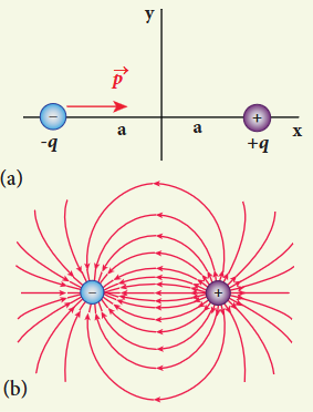
The electric dipole moment vector lies along the line joining two charges and is directed from \(-q\) to \(+q\). The SI unit of dipole moment is coulomb metre (Cm).
- For simplicity, the two charges are placed on the \(x\)-axis. Even if the two charges are placed on \(y\) or \(z\)-axis, dipole moment will point from \(-q\) to \(+q\).
- The magnitude of the electric dipole moment is equal to the product of the magnitude of one of the charges and the distance between them,
- Though the electric dipole moment for two equal and opposite charges is defined, it is possible to define and calculate the electric dipole moment for a collection of point charges. The electric dipole moment for a collection of \(n\) point charges is given by
where \(\bar{r}_{i}\) is the position vector of charge \(q_{i}\) from the origin.
EXAMPLE 1.10
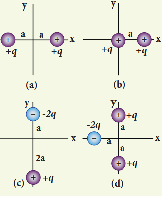
Calculate the electric dipole moment for the following charge configurations.
Solution
Case (a) The position vector for the \(+q\) on the positive \(x\)-axis is \(a\hat{i}\) and position vector for the \(+q\) charge the negative \(x\) axis is \(-a\hat{i}\). So the dipole moment is,
$$ \bar{p} = (+q)(a\hat{i}) + (+q)(-a\hat{i}) = 0 $$Case (b) In this case one charge is placed at the origin, so its position vector is zero. Hence only the second charge \(+q\) with position vector \(a\hat{i}\) contributes to the dipole moment, which is \(\bar{p} = qa\hat{i}\).
From both cases (a) and (b), we can infer that in general the electric dipole moment depends on the choice of the origin and charge configuration. But for one special case, the electric dipole moment is independent of the origin. If the total charge is zero, then the electric dipole moment will be the same irrespective of the choice of the origin. It is because of this reason that the electric dipole moment of an electric dipole (total charge is zero) is always directed from \(-q\) to \(+q\), independent of the choice of the origin.
Case (c) \(\bar{p} = (-2q)a\hat{j} + q(2a)(-\hat{j}) = -4qa\hat{j}\). Note that in this case \(\bar{p}\) is directed from \(-2q\) to \(+q\).
Case (d) \(\bar{p} = -2qa(-\hat{i}) + qa\hat{j} + qa(-\hat{j}) = 2qa\hat{i}\)
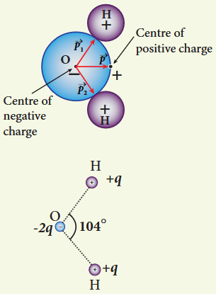
The water molecule \(\mathrm{H}_{2}\mathrm{O}\) has this charge configuration. The water molecule has three atoms (two H atom and one O atom). The centres of positive (H) and negative (O) charges of a water molecule lie at different points, hence it possess permanent dipole moment. The electric dipole moment \(\bar{p}\) is directed from centre of negative charge to the centre of positive charge.
Electric field due to a dipole#
Case (i) Electric field due to an electric dipole at points on the axial line
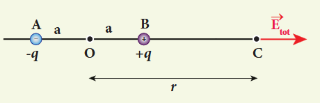
Consider an electric dipole placed on the \(x\)-axis as shown in Figure 1.15. A point C is located at a distance of \(r\) from the midpoint O of the dipole on the axial line.
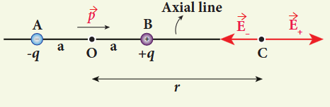
The electric field at a point C due to \(+q\) is \(\bar{E}_{+} = \frac{1}{4\pi\epsilon_{0}}\frac{q}{\left(r - a\right)^{2}}\) along BC
Since the electric dipole moment vector \(\vec{p}\) is from \(-q\) to \(+q\) and is directed along BC, the above equation is rewritten as
$$ \bar{E}_{+} = \frac{1}{4\pi\epsilon_{0}}\frac{q}{\left(r - a\right)^{2}}\hat{p} \quad (1.13) $$where \(\hat{p}\) is the electric dipole moment unit vector from \(-q\) to \(+q\)
The electric field at a point C due to \(-q\) is
$$ \bar{E}_{-} = -\frac{1}{4\pi\epsilon_{0}}\frac{q}{\left(r + a\right)^{2}}\hat{p} \quad (1.14) $$Since \(+q\) is located closer to the point C than \(-q\), \(\bar{E}_{+}\) is stronger than \(\bar{E}_{-}\). Therefore, the length of the \(\bar{E}_{+}\) vector is drawn larger than that of \(\bar{E}_{-}\) vector.
The total electric field at point C is calculated using the superposition principle of the electric field.
$$ \bar{E}_{tot} = \bar{E}_{+} + \bar{E}_{-} $$$$ = \frac{1}{4\pi\epsilon_{0}}\frac{q}{\left(r - a\right)^{2}}\hat{p} - \frac{1}{4\pi\epsilon_{0}}\frac{q}{\left(r + a\right)^{2}}\hat{p} $$$$ \bar{E}_{tot} = \frac{q}{4\pi\epsilon_{0}}\left(\frac{1}{\left(r - a\right)^{2}} - \frac{1}{\left(r + a\right)^{2}}\right)\hat{p} \quad (1.15) $$$$ \bar{E}_{tot} = \frac{1}{4\pi\epsilon_{0}} q\left(\frac{4ra}{\left(r^{2} - a^{2}\right)^{2}}\right)\hat{p} \quad (1.16) $$Note that the total electric field is along \(\bar{E}_{+}\) since \(+q\) is closer to C than \(-q\).
If the point C is very far away from the dipole \((r \gg a)\). Then under this limit the term \(\left(r^{2} - a^{2}\right)^{2} = r^{4}\). Substituting this into equation (1.16), we get
$$ \bar{E}_{tot} = \frac{1}{4\pi\epsilon_{0}}\left(\frac{4aq}{r^{3}}\right)\hat{p} \quad (r \gg a) $$$$ \text{since } 2aq\hat{p} = \bar{p} $$$$ \bar{E}_{tot} = \frac{1}{4\pi\epsilon_{0}}\frac{2\bar{p}}{r^{3}} \quad (r \gg a) $$If the point C is chosen on the left side of the dipole, the total electric field is still in the direction of \(\bar{p}\).
Case (ii) Electric field due to an electric dipole at a point on the equatorial plane
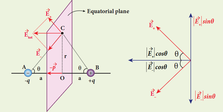
Consider a point C at a distance \(r\) from the midpoint O of the dipole on the equatorial plane as shown in Figure 1.17. Since the point C is equidistant from \(+q\) and \(-q\), the magnitude of the electric fields at C due to \(+q\) and \(-q\) are the same. The direction of \(\bar{E}_{+}\) is along BC and the direction of \(\bar{E}_{-}\) is along CA. \(\bar{E}_{+}\) and \(\bar{E}_{-}\) can be resolved into two components; one component parallel to the dipole axis and the other perpendicular to it. Since perpendicular components \(\left|\bar{E}_{+}\right|\sin \theta\) and \(\left|\bar{E}_{-}\right|\sin \theta\) are equal in magnitude and oppositely directed, they cancel each other. The magnitude of the total electric field at point C is the sum of the parallel components of \(\bar{E}_{+}\) and \(\bar{E}_{-}\) and its direction is along \(-\hat{p}\) as shown.
The magnitudes \(\bar{E}_{+}\) and \(\bar{E}_{-}\) are the same and are given by
$$ \left|\bar{E}_{+}\right| = \left|\bar{E}_{-}\right| = \frac{1}{4\pi\epsilon_{0}}\frac{q}{\left(r^{2} + a^{2}\right)} \quad (1.19) $$By substituting equation (1.19) into equation (1.18), we get
$$ \bar{E}_{tot} = -\frac{1}{4\pi\epsilon_{0}}\frac{2q\cos\theta}{\left(r^{2} + a^{2}\right)}\hat{p} $$$$ = -\frac{1}{4\pi\epsilon_{0}}\frac{2qa}{\left(r^{2} + a^{2}\right)^{3/2}}\hat{p} \quad (\text{since }\cos \theta = \frac{a}{\sqrt{r^{2} + a^{2}}}) $$$$ \bar{E}_{tot} = -\frac{1}{4\pi\epsilon_{0}}\frac{\bar{p}}{\left(r^{2} + a^{2}\right)^{\frac{3}{2}}} \quad (\text{since }\bar{p} = 2qa\hat{p}) \quad (1.20) $$At very large distances \((r \gg a)\), the equation (1.20) becomes
$$ \bar{E}_{tot} = -\frac{1}{4\pi\epsilon_{0}}\frac{\bar{p}}{r^{3}} \quad (r \gg a) \quad (1.21) $$Important inferences#
(i) From equations (1.17) and (1.21), it is inferred that for very large distances, the magnitude of the electric field at point on the dipole axis is twice the magnitude of the electric field at the point at the same distance on the equatorial plane. The direction of the electric field at points on the dipole axis is directed along the direction of dipole moment vector \(\bar{p}\) but at points on the equatorial plane it is directed opposite to the dipole moment vector, that is along \(-\bar{p}\).
(ii) At very large distances, the electric field due to a dipole varies as \(\frac{1}{r^{3}}\). Note that for a point charge, the electric field varies as \(\frac{1}{r^{2}}\).This implies that the electric field due to a dipole at very large distances goes to zero faster than the electric field due to a point charge. The reason for this behavior is that at very large distance, the two charges appear to be close to each other and neutralize each other.
(iii) The equations (1.17) and (1.21) are valid only at very large distances (r»a). Suppose the distance 2a approaches zero and q approaches infinity such that the product of 2aq = p is finite, then the dipole is called a point dipole. For such point dipoles, equations (1.17) and (1.21) are exact and hold true for any r.
Torque experienced by an electric dipole in the uniform electric field#
Consider an electric dipole of dipole moment \(\vec{p}\) placed in a uniform electric field \(\vec{E}\) whose field lines are equally spaced and point in the same direction. The charge \(+q\) will experience a force \(q\vec{E}\) in the direction of the field and charge \(-q\) will experience a force \(-q\vec{E}\) in a direction opposite to the field. Since the external field \(\vec{E}\) is uniform, the total force acting on the dipole is zero. These two forces acting at different points will constitute a couple and the dipole experience a torque. This torque tends to rotate the dipole. (Note that electric field lines of a uniform field are equally spaced and point in the same direction).
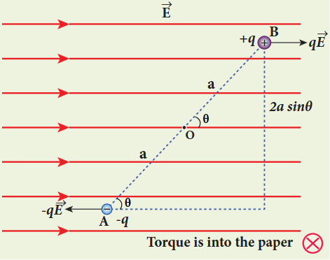
The total torque on the dipole about the point O
$$ \vec{\tau} = \overline{OA}\times (-q\vec{E}) + \overline{OB}\times q\vec{E} \quad (1.22) $$Using right-hand corkscrew rule (Refer XI, volume 1, unit 2), it is found that total torque is perpendicular to the plane of the paper and is directed into it.
The magnitude of the total torque
$$ \tau = \left|\overline{OA}\right|\left|(-q\vec{E})\right|\sin \theta + \left|\overline{OB}\right|\left|q\vec{E}\right|\sin \theta $$$$ \tau = qE \cdot 2a\sin \theta \quad (1.23) $$where \(\theta\) is the angle made by \(\vec{p}\) with \(\vec{E}\). Since \(p = 2aq\), the torque is written in terms of the vector product as
$$ \vec{\tau} = \vec{p}\times \vec{E} \quad (1.24) $$The magnitude of this torque is \(\tau = pE\sin \theta\) and is maximum when \(\theta = 90^{\circ}\)
This torque tends to rotate the dipole and align it with the electric field \(\vec{E}\). Once \(\vec{p}\) is aligned with \(\vec{E}\), the total torque on the dipole becomes zero.
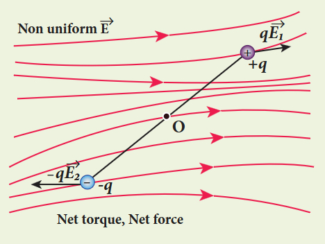
If the electric field is not uniform, then the force experienced by \(+q\) is different from that experienced by \(-q\). In addition to the torque, there will be net force acting on the dipole.
EXAMPLE 1.11
A sample of HCl gas is placed in a uniform electric field of magnitude \(3\times 10^{4}\mathrm{N C^{-1}}\). The dipole moment of each HCl molecule is \(3.4\times 10^{-30}\mathrm{Cm}\). Calculate the maximum torque experienced by each HCl molecule.
Solution
The maximum torque experienced by the dipole is when it is aligned perpendicular to the applied field.
$$ \tau_{\mathrm{max}} = pE\sin 90^{\circ} = 3.4\times 10^{-30}\times 3\times 10^{4} $$$$ \tau_{\mathrm{max}} = 10.2\times 10^{-26}\mathrm{Nm} $$Microwave oven works on the principle of torque acting on an electric dipole. The food we consume has water molecules which are permanent electric dipoles. Oven produces microwaves that are oscillating electromagnetic fields and produce torque on the water molecules. Due to this torque on each water molecule, the molecules rotate very fast and produce thermal energy. Thus, heat generated is used to heat the food.